What?

When PyTorch builds a computation graph of your ML model, it tries many different things to make it fast and memory efficient. One technique is to take a joint forward and backward computation graph and choose which operations should be saved (stored in a memory and reused) and which operations should be recomputed. Each operation takes some time to run and takes up some memory if stored and we only can use a limited amount of memory.

0/1 Knapsack problem

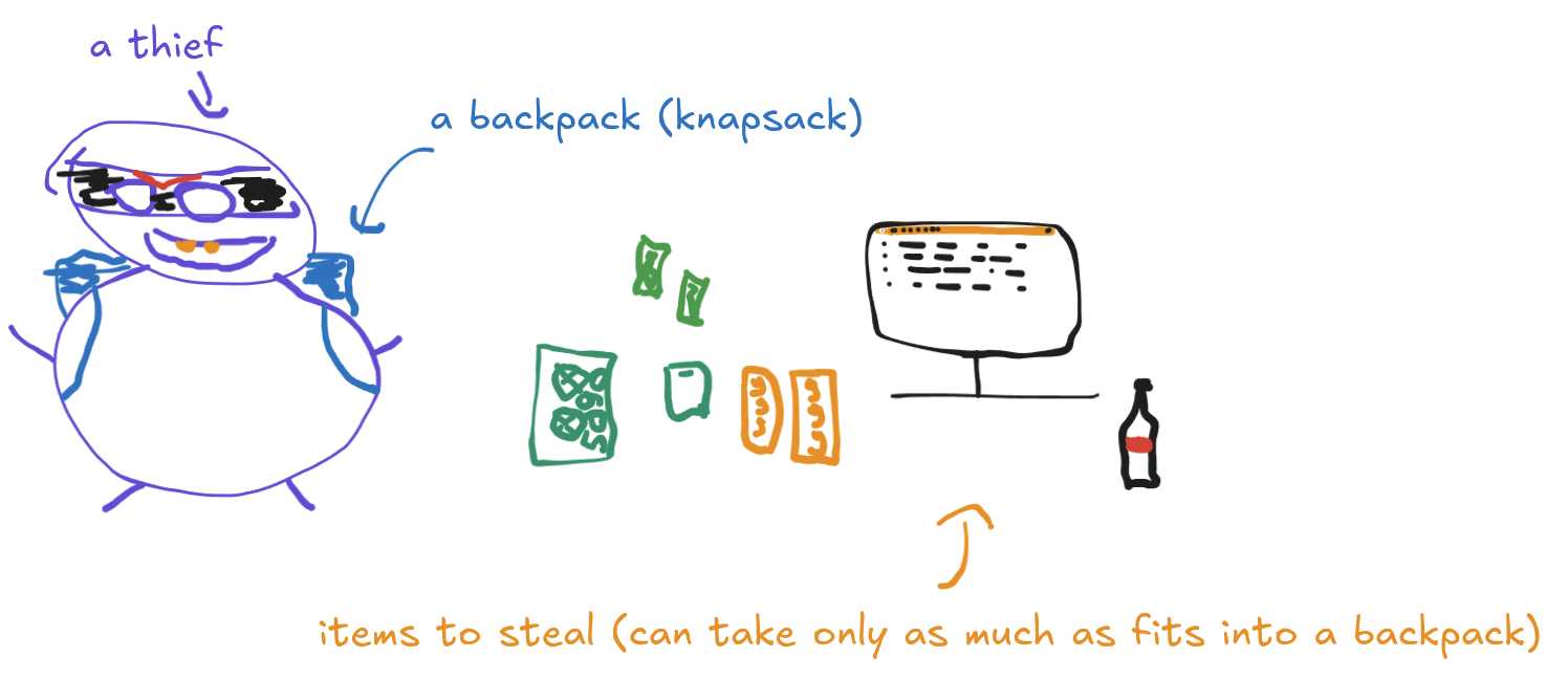
Imagine you are a thief and you just broke into a place with many valuable things inside. You have a knapsack that can carry up to 10 kilograms. You want to maximize the value of things you steal. Ideally, you'd just take all of them. But if you put more than 10kg to your knaspack, it will break and you will get away with nothing. Alternatively, you can use some heuristics to pick the items (like take only small items or only green ones), but then your solution might not be optimal - you will steal some value, but perhaps less than what you could gain in an optimal choice. For your rescue, there come 0/1 knapsack solvers. There are different algorithms that compute optimal items choice within a given capacity (max weight of things in a knapsack) and given a list of items, where each of items has a value and a cost (weight). In PyTorch, this is what we actually do, which is: within a RAM budget (knapsack capacity), we choose which operations (items) should be saved to the memory to maximize the time savings in runtime (value).

dp_knapsack

Currently, the default implementation of knapsack solver in PyTorch is dp_knapsack, which is a dynamic programming approach to solving 0/1 knapsack. The algoritmh is actually simple once you understand it. It helps a lot if you have had a prior experience with dynamic programming (I do not). Look at this nice GIF from Wikipedia:

By RDSEED - Own work, CC BY-SA 4.0, Link

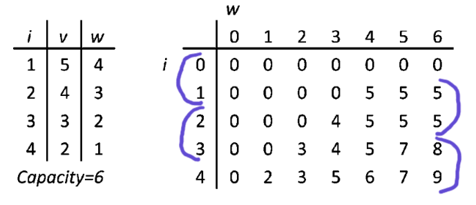
On the left, there is a list of 4 items. i is an index, v is a value and w is a weight. Units irrelevant. Capacity is 6. That's why on the right side there are 6 columns (each column is a part of total capacity) and 4 rows (one per item). Ok, actually there are 7 and 5, because of padding with zeros, but that's only for a computation convenience (every row and column has a parent, index arithmetic gets much easier). You could actually do it without padding, but I tried and fallbacked to padding anyways, because index arithmetic was a bit annoying. The table on the right is called a DP table. It's where the computation happens.

Building a DP table

DP 0/1 Knapsack algorithm goes like this: get an item. In a DP table, go through a corresponding row, column by column and compare your item's value to value in current DP table cell (row, column; current column index is current max weight (capacity) of your knapsack). If your item's weight is bigger than current column's index, move on to the next column. If your item weight is equal to a column index and your item value is higher than current cell, replace the cell with your item value. If your item weight is smaller than column index and it fits in a spare capacity, add it to the cell's value (a free capacity is current capacity minus capacity of picked items). Repeat until you iterate through all the items. At this point, you learn what is the maximum value you can get within the weight budget. If our goal would be to measure a max possible value, then we would stop at this point. Unfortunately, we want to know more.

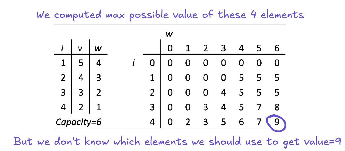
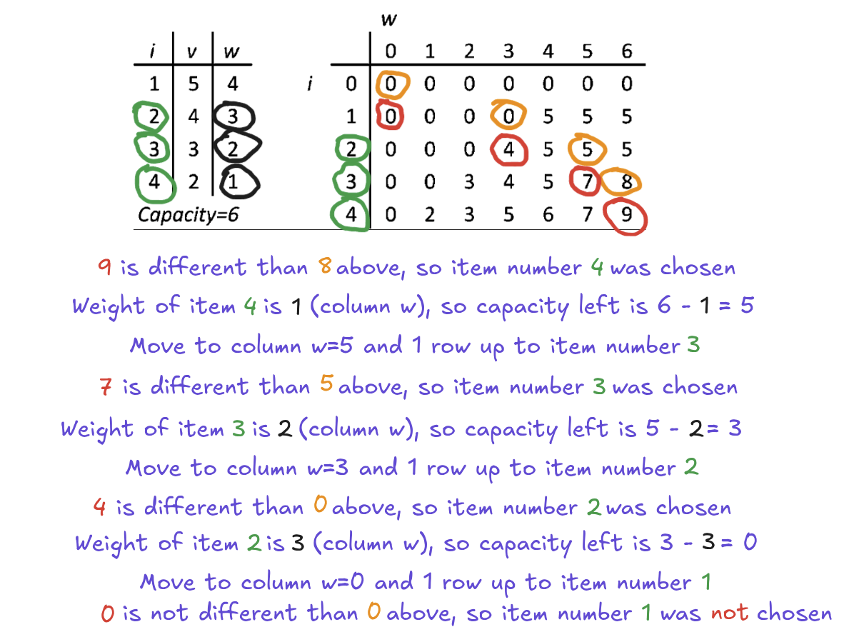
Backtracking

We need to know which items we should take to get this max possible value. So in case of PyTorch, which operations which we should save to memory and which operations we should recompute. To find out which items contribute to the max value (in other words, which items were chosen during building DP table), we need to go backwards through the DP table. We go from the last row and last column upward. We compare a cell with a cell above (same column, previous row). If they are different, then the current item contributes to the max value - because each row corresponds to a single item. If they are equal, this item will not be stored in a memory and becomes recomputable. Now, we traverse the DP table upward. If the item was chosen, we move upward by a single row and we move the position of the current cell to the left by the weight of the chosen item. If item wasn't chosen, we move upward by a single row and we start on the same position as previously. Repeat until we get to the top of the DP table.

Optimization

This solver works correctly. It provides an exact solution and for most of the time you don't need anything better. By better I mean 1. faster and 2. less memory hungry. Because look again at the algorithm and the GIF above. There are a few issues with it. To get a result, we allocate a full 2D table of shape=(number of items, max_weight), which is not great. Horace He (Chillee) who originally built a great part of (all of?) the memory planning in PyTorch left a note in the DP knapsack solver code:

# TODO(chilli): I think if needed, this memory can be optimized with sliding
# window trick + Hirschberg trick:
# https://codeforces.com/blog/entry/47247?#comment-316200

What he proposes are two optimizations.

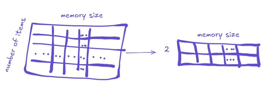
Sliding window

Window trick means that instead of building the a DP table, we slide over a table and use only a previous row and a current row. When moving to the next row, next becomes a new current and old current becomes a previous row. This improvement alone would be enough, if we wanted to just compute the max value of items out of our list, within a given capacity. But again, we need to know which items contribute to this max value. That's why Horace suggested using a sliding window together with Hirschberg trick.

Hirschberg trick

It's a divide and conquer approach, kinda similar to quicksort, because you split problem into smaller ones and solve them and continue splitting until you solve the whole problem. The main benefit of Hirschberg trick for usis that it gets rid of backtracking.

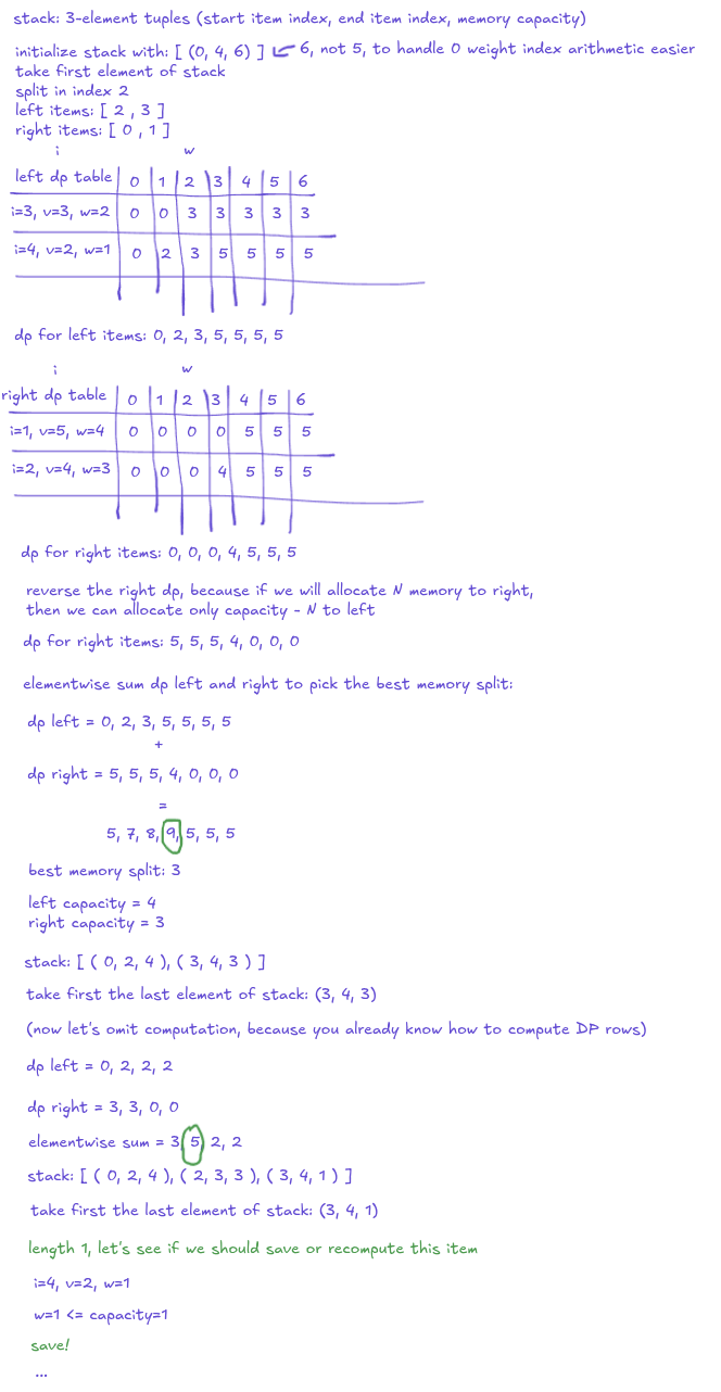
From an implementation perspective, I sort of do a recursion here, but without putting new frames on the stack. I have a Python list that I use as an explicit stack (last in, first out). The list stores a range of item indexes and a currently available capacity. We start with all the items and all the capacity. Then the algo goes like this: First, we pop an item from the stack. If it's a single item (item index range end - start = 1), check if item's weight fits in the available capacity. If yes, include it in saved items, if not, include it in recomputable items. This part is imo the biggest strength of Hirschberg algorithm for us - because you can see now that we won't need a backtracking, since we build saved and recomputable lists inside the algorithm. No need to build it afterwards, unlike in original 0/1 DP knapsack algorithm. If the items range is bigger than 1, split the items into a two parts and for each of them compute a DP table. We don't want to build a full DP table, so we do the sliding window trick here and reuse a current and previous DP row to compute the final DP row.

Once we have both left and right DP rows, add them together. Find the position of the highest value. It will be the new splitting point for our memory. Now we split the memory into two, using this newly computed position and we run the algorithm again, using both memory and items split. Repeat until done. Btw. It might happen that one of the splitted parts will be empty. It might happen when the best split is either the first or last item. That's completely legit, we just skip such an stack frame and move on.

Here is a great explanation with drawings step by step of Hirschberg algo by KokiYmgch on CodeForces

So, is dp_knapsack_sliding_hirschberg THE solver now?

No. Look - with these two optimizations combined, we can decrease the DP table size from shape=(number of items, max weight) to shape=(2, max weight), effectively reducing a peak memory by a factor of 20x - on my machine with 64GB RAM dp_knapsack crashes on problems with 100 items, while dp_knapsack_sliding_hirschberg is able to handle problems with 2000 items within this RAM budget. We also gain some runtime speedup, roughly 37%, but I didn't measure it very rigorously, though. That being said - if you don't mind using SciPy, then you probably should use ilp_knapsack instead. It's MUCH faster than any existing DP knapsack implementation in PyTorch. It's a bit slower than a greedy algorithm, but still very fast, yet unlike greedy and similarly to both DP solvers, it provides an exact solution.

How to pick a right solver for you

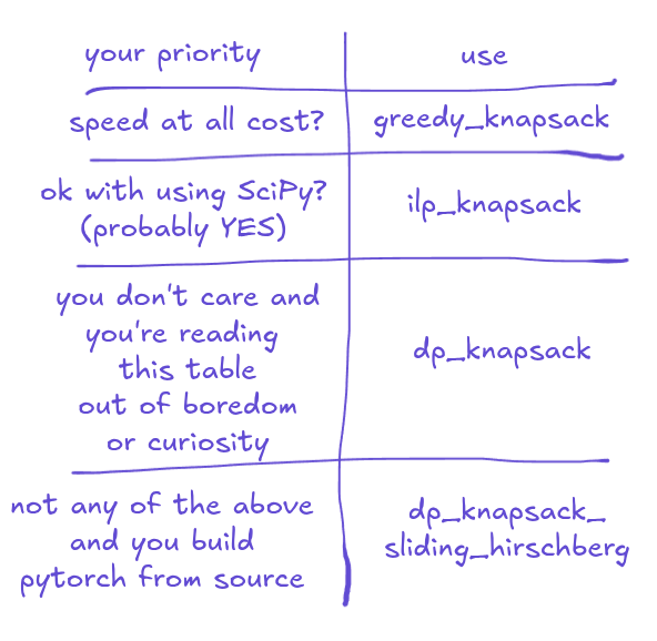
If you care about speed above correctness, use greedy_knapsack.

Else if you're ok with pulling SciPy into project, use ilp_knapsack.

Else if you install PyTorch from a package manager, noop - PyTorch will use dp_knapsack, which is a default solver and you don't need to do anything.

Else use dp_knapsack_sliding_hirschberg.

How to use dp_knapsack_sliding_hirschberg

It's not released in an official version yet, so if you don't want to build PyTorch from the main branch and you want to use it, you need to wait a bit. If you're a developer or an early adopter and you build PyTorch from source, you can use the main branch and just paste the snippet below early in your PyTorch code and you're set up

import torch
import torch._functorch.config as fconfig
fconfig.activation_memory_budget_solver = fconfig.dp_knapsack_sliding_hirschberg

If you spot any bugs when using dp_knapsack_sliding_hirschberg, pls register an issue and tag me @jmaczan and I'll hop on to solve it.

Thanks to Edward Yang for a code review and a merge and thanks to you for reading

← main page

 . 
  .
...